Cox–Ingersoll–Ross model

Three trajectories of CIR Processes

In mathematical finance, the Cox–Ingersoll–Ross model (or CIR model) describes the evolution of interest rates. It is a type of "one factor model" (short rate model) as it describes interest rate movements as driven by only one source of market risk. The model can be used in the valuation of interest rate derivatives. It was introduced in 1985 by John C. Cox, Jonathan E. Ingersoll and Stephen A. Ross as an extension of the Vasicek model.

The model

CIR process

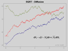
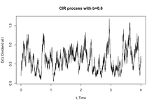
The CIR model specifies that the instantaneous interest rate follows the stochastic differential equation, also named the CIR Process:

dr_{t}=a(b-r_{t})\,dt+\sigma {\sqrt {r_{t}}}\,dW_{t}

where $W_{t}$ is a Wiener process (modelling the random market risk factor) and $a$ , $b$ , and $\sigma \,$ are the parameters. The parameter $a$ corresponds to the speed of adjustment, $b$ to the mean and $\sigma \,$ to volatility. The drift factor, $a(b-r_{t})$ , is exactly the same as in the Vasicek model. It ensures mean reversion of the interest rate towards the long run value $b$ , with speed of adjustment governed by the strictly positive parameter $a$ .

The standard deviation factor, $\sigma {\sqrt {r_{t}}}$ , avoids the possibility of negative interest rates for all positive values of $a$ and $b$ . An interest rate of zero is also precluded if the condition

2ab\geq \sigma ^{2}\,

is met. More generally, when the rate ( $r_{t}$ ) is close to zero, the standard deviation ( $\sigma {\sqrt {r_{t}}}$ ) also becomes very small, which dampens the effect of the random shock on the rate. Consequently, when the rate gets close to zero, its evolution becomes dominated by the drift factor, which pushes the rate upwards (towards equilibrium).

This process can be defined as a sum of squared Ornstein–Uhlenbeck process. The CIR is an ergodic process, and possesses a stationary distribution. The same process is used in the Heston model to model stochastic volatility.

Distribution

Future distribution

The distribution of future values of a CIR process can be computed in closed form:

r_{{t+T}}={\frac {Y}{2c}}

where $c={\frac {2a}{(1-e^{{-aT}})\sigma ^{2}}}$ , and Y is a non-central Chi-Squared distribution with ${\frac {4ab}{\sigma ^{2}}}$ degrees of freedom and non-centrality parameter $2cr_{t}e^{{-aT}}$ . Formally the probability density function is:

f(r_{{t+T}};r_{t},a,b,\sigma )=c\,e^{{-u-v}}\left({\frac {v}{u}}\right)^{{q/2}}I_{{q}}(2{\sqrt {uv}})

where $q={\frac {2ab}{\sigma ^{2}}}-1$ , $u=cr_{t}e^{{-aT}}$ , $v=cr_{{t+T}}$ , and $I_{q}(2{\sqrt {uv}})$ is modified Bessel function of the first kind of order $q$ .

Asymptotic distribution

Due to mean reversion, as time becomes large, the distribution of $r_{{\infty }}$ will approach a gamma distribution with the probability density of:

f(r_{{\infty }};a,b,\sigma )={\frac {\omega ^{\nu }}{\Gamma (\nu )}}r_{\infty }^{{\nu -1}}e^{{-\omega r_{\infty }}}

where $\omega =2a/\sigma ^{2}$ and $\nu =2ab/\sigma ^{2}$ .

Properties

Mean reversion,
Level dependent volatility ( $\sigma {\sqrt {r_{t}}}$ ),
For given positive $r_{0}$ the process will never touch zero, if $2ab\geq \sigma ^{2}$ ; otherwise it can occasionally touch the zero point,
$E[r_{t}|r_{0}]=r_{0}e^{{-at}}+b(1-e^{{-at}})$ , so long term mean is $b$ ,
$Var[r_{t}|r_{0}]=r_{0}{\frac {\sigma ^{2}}{a}}(e^{{-at}}-e^{{-2at}})+{\frac {b\sigma ^{2}}{2a}}(1-e^{{-at}})^{2}$ .

Calibration

Ordinary least squares

The continuous SDE can be discretized as follows

$r_{t+\Delta t}-r_{t}=a(b-r_{t})\,\Delta t+\sigma \,{\sqrt {r_{t}\Delta t}}\epsilon _{t}$ ,

which is equivalent to

${\frac {r_{t+\Delta t}-r_{t}}{{\sqrt {r}}_{t}}}={\frac {ab\Delta t}{{\sqrt {r}}_{t}}}-a{\sqrt {r}}_{t}\Delta t+\sigma \,{\sqrt {\Delta t}}\epsilon _{t}$ , provided $\epsilon _{t}$ is n.i.i.d. (0,1). This equation can be used for a linear regression.

Martingale estimation
Maximum likelihood

Simulation

Stochastic simulation of the CIR process can be achieved using two variants:

Discretization
Exact

Bond pricing

Under the no-arbitrage assumption, a bond may be priced using this interest rate process. The bond price is exponential affine in the interest rate:

P(t,T)=A(t,T)\exp(-B(t,T)r_{t})\!

where

A(t,T)=\left({\frac {2h\exp((a+h)(T-t)/2)}{2h+(a+h)(\exp((T-t)h)-1)}}\right)^{{2ab/\sigma ^{2}}}

B(t,T)={\frac {2(\exp((T-t)h)-1)}{2h+(a+h)(\exp((T-t)h)-1)}}

h={\sqrt {a^{2}+2\sigma ^{2}}}

Extensions

Time varying functions replacing coefficients can be introduced in the model in order to make it consistent with a pre-assigned term structure of interest rates and possibly volatilities. The most general approach is in Maghsoodi (1996). A more tractable approach is in Brigo and Mercurio (2001b) where an external time-dependent shift is added to the model for consistency with an input term structure of rates. A significant extension of the CIR model to the case of stochastic mean and stochastic volatility is given by Lin Chen (1996) and is known as Chen model. A CIR process is a special case of a basic affine jump diffusion, which still permits a closed-form expression for bond prices.

References

Hull, John C. (2003). Options, Futures and Other Derivatives. Upper Saddle River, NJ: Prentice Hall. ISBN 0-13-009056-5.
Cox, J.C., J.E. Ingersoll and S.A. Ross (1985). "A Theory of the Term Structure of Interest Rates". Econometrica. 53: 385–407. doi:10.2307/1911242.
Maghsoodi, Y. (1996). "Solution of the extended CIR Term Structure and Bond Option Valuation". Mathematical Finance (6): 89–109.
Damiano Brigo; Fabio Mercurio (2001). Interest Rate Models — Theory and Practice with Smile, Inflation and Credit (2nd ed. 2006 ed.). Springer Verlag. ISBN 978-3-540-22149-4.
Brigo, Damiano; Fabio Mercurio (2001b). "A deterministic-shift extension of analytically tractable and time-homogeneous short rate models". Finance & Stochastics. 5 (3): 369–388.
Open Source library implementing the CIR process in python

Bond market

Bond Debenture Fixed income

Types of bonds by issuer	Agency bond Corporate bond Senior debt Subordinated debt Distressed debt Emerging market debt Government bond Municipal bond

Types of bonds by payout	Accrual bond Auction rate security Callable bond Commercial paper Contingent convertible bond Convertible bond Exchangeable bond Extendible bond Fixed rate bond Floating rate note High-yield debt Inflation-indexed bond Inverse floating rate note Perpetual bond Puttable bond Reverse convertible securities Zero-coupon bond

Bond valuation	Clean price Convexity Coupon Credit spread Current yield Dirty price Duration I-spread Mortgage yield Nominal yield Risk-free bond Yield to maturity Z-spread

Securitized products	Asset-backed security Collateralized debt obligation Collateralized mortgage obligation Commercial mortgage-backed security Mortgage-backed security Yield-curve spread

Bond options	Callable bond Convertible bond Embedded option Exchangeable bond Extendible bond Option-adjusted spread Puttable bond

Institutions	Commercial Mortgage Securities Association (CMSA) International Capital Market Association (ICMA) Securities Industry and Financial Markets Association (SIFMA)

Stochastic processes

Discrete time	Bernoulli process Branching process Chinese restaurant process Galton–Watson process Independent and identically distributed random variables Markov chain Moran process Random walk Loop-erased Self-avoiding

Continuous time	Bessel process Birth–death process Brownian motion Bridge Excursion Fractional Geometric Meander Cauchy process Contact process Continuous-time random walk Cox process Diffusion process Empirical process Feller process Fleming–Viot process Gamma process Hunt process Interacting particle systems Itô diffusion Itô process Jump diffusion Jump process Lévy process Local time Markov additive process McKean–Vlasov process Ornstein–Uhlenbeck process Poisson process Compound Non-homogeneous Point process Schramm–Loewner evolution Semimartingale Sigma-martingale Stable process Superprocess Telegraph process Variance gamma process Wiener process Wiener sausage

Both	Branching process Galves–Löcherbach model Gaussian process Hidden Markov model (HMM) Markov process Martingale Differences Local Sub- Super- Random dynamical system Regenerative process Renewal process Stochastic chains with memory of variable length White noise

Fields and other	Dirichlet process Gaussian random field Gibbs measure Hopfield model Ising model Potts model Boolean network Markov random field Percolation Pitman–Yor process Point process Cox Poisson Random field Random graph

Time series models	Autoregressive conditional heteroskedasticity (ARCH) model Autoregressive integrated moving average (ARIMA) model Autoregressive (AR) model Autoregressive–moving-average (ARMA) model Generalized autoregressive conditional heteroskedasticity (GARCH) model Moving-average (MA) model

Financial models	Black–Derman–Toy Black–Karasinski Black–Scholes Chen Constant elasticity of variance (CEV) Cox–Ingersoll–Ross (CIR) Garman–Kohlhagen Heath–Jarrow–Morton (HJM) Heston Ho–Lee Hull–White LIBOR market Rendleman–Bartter SABR volatility Vašíček Wilkie

Actuarial models	Bühlmann Cramér–Lundberg Risk process Sparre–Anderson

Queueing models	Bulk Fluid Generalized queueing network M/G/1 M/M/1 M/M/c

Properties	Càdlàg paths Continuous Continuous paths Ergodic Exchangeable Feller-continuous Gauss–Markov Markov Mixing Piecewise deterministic Predictable Progressively measurable Self-similar Stationary Time-reversible

Limit theorems	Central limit theorem Donsker's theorem Doob's martingale convergence theorems Ergodic theorem Fisher–Tippett–Gnedenko theorem Large deviation principle Law of large numbers (weak/strong) Law of the iterated logarithm Maximal ergodic theorem Sanov's theorem

Inequalities	Burkholder–Davis–Gundy Doob's martingale Kunita–Watanabe

Tools	Cameron–Martin formula Convergence of random variables Doléans-Dade exponential Doob decomposition theorem Doob–Meyer decomposition theorem Doob's optional stopping theorem Dynkin's formula Feynman–Kac formula Filtration Girsanov theorem Infinitesimal generator Itô integral Itô's lemma Kolmogorov continuity theorem Kolmogorov extension theorem Lévy–Prokhorov metric Malliavin calculus Martingale representation theorem Optional stopping theorem Prokhorov's theorem Quadratic variation Reflection principle Skorokhod integral Skorokhod's representation theorem Skorokhod space Snell envelope Stochastic differential equation Tanaka Stopping time Stratonovich integral Uniform integrability Usual hypotheses Wiener space Classical Abstract

Disciplines	Actuarial mathematics Econometrics Ergodic theory Extreme value theory (EVT) Large deviations theory Mathematical finance Mathematical statistics Probability theory Queueing theory Renewal theory Ruin theory Statistics Stochastic analysis Time series analysis Machine learning

List of topics Category

This article is issued from Wikipedia - version of the 12/3/2016. The text is available under the Creative Commons Attribution/Share Alike but additional terms may apply for the media files.