Point set registration

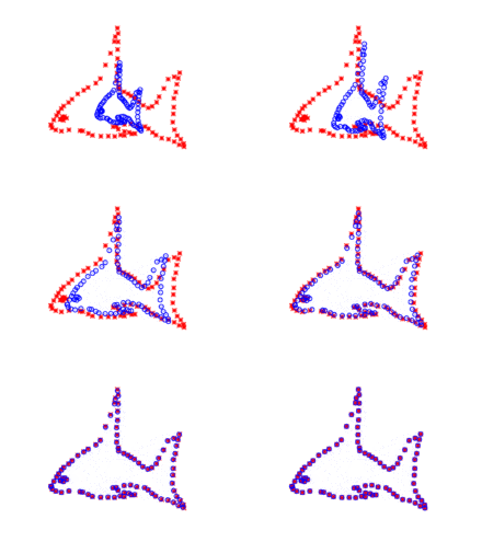
Point set registration is the process of aligning two point sets. Here, the blue fish is being registered to the red fish.

In computer vision and pattern recognition, point set registration, also known as point matching, is the process of finding a spatial transformation that aligns two point sets. The purpose of finding such a transformation includes merging multiple data sets into a globally consistent model, and mapping a new measurement to a known data set to identify features or to estimate its pose. A point set may be raw data from 3D scanning or an array of rangefinders. For use in image processing and feature-based image registration, a point set may be a set of features obtained by feature extraction from an image, for example corner detection. Point set registration is used in optical character recognition^[1]^[2] and aligning data from magnetic resonance imaging with computer aided tomography scans.^[3]^[4]

Overview of problem

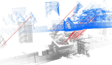
Data from two 3D scans of the same environment need to be aligned using point set registration.

Data from above, registered successfully using a variant of iterative closest point.

The problem may be summarized as follows:^[5] Let $\lbrace {\mathcal {M}},{\mathcal {S}}\rbrace$ be two finite size point sets in a finite-dimensional real vector space $\mathbb {R} ^{d}$ , which contain $M$ and $N$ points respectively. The problem is to find a transformation to be applied to the moving "model" point set ${\mathcal {M}}$ such that the difference between ${\mathcal {M}}$ and the static "scene" set ${\mathcal {S}}$ is minimized. In other words, a mapping from $\mathbb {R} ^{d}$ to $\mathbb {R} ^{d}$ is desired which yields the best alignment between the transformed "model" set and the "scene" set. The mapping may consist of a rigid or non-rigid transformation. The transformation model may be written as $T$ where the transformed, registered model point set is:

$T({\mathcal {M}})$

(1)

It is useful to define an optimization parameter $\theta$ :

$T({\mathcal {M}},\theta )$

(2)

such that it is clear that the optimizing algorithm adjusts $\theta$ . Depending on the problem and number of dimensions, there may be more such parameters. The output of a point set registration algorithm is therefore the transformation parameter $\theta$ of model $T$ so that ${\mathcal {M}}$ is optimally aligned to ${\mathcal {S}}$ .

In convergence, it is desired for the distance between the two point sets to reach a global minimum. This is difficult without exhausting all possible transformations, so a local minimum suffices. The distance function between a transformed model point set $T({\mathcal {M}})$ and the scene point set ${\mathcal {S}}$ is given by some function $\operatorname {dist}$ . A simple approach is to take the square of the Euclidean distance for every pair of points:

$\operatorname {dist} (T({\mathcal {M}}),{\mathcal {S}})=\sum _{m\in T({\mathcal {M}})}\sum _{s\in {\mathcal {S}}}(m-s)^{2}$

(3)

Minimizing such a function in rigid registration is equivalent to solving a least squares problem. However, this function is sensitive to outlier data and consequently algorithms based on this function tend to be less robust against noisy data. A more robust formulation of the cost function uses some robust function $g$ :

$\operatorname {dist} _{\operatorname {robust} }(T({\mathcal {M}}),{\mathcal {S}})=\sum _{m\in T({\mathcal {M}})}\sum _{s\in {\mathcal {S}}}g((m-s)^{2})$

(4)

Such a formulation is known as an M-estimator. The robust function $g$ is chosen such that the local configuration of the point set is insensitive to distant points, hence making it robust against outliers and noise.^[6]

Rigid registration

Given two point sets, rigid registration yields a rigid transformation which maps one point set to the other. A rigid transformation is defined as a transformation that does not change the distance between any two points. Typically such a transformation consists of translation and rotation.^[2] In rare cases, the point set may also be mirrored.

Non-rigid registration

Given two point sets, non-rigid registration yields a non-rigid transformation which maps one point set to the other. Non-rigid transformations include affine transformations such as scaling and shear mapping. However, in the context of point set registration, non-rigid registration typically involves nonlinear transformation. If the eigenmodes of variation of the point set are known, the nonlinear transformation may be parametrized by the eigenvalues.^[7] A nonlinear transformation may also be parametrized as a thin plate spline.^[1]^[7]

Point set registration algorithms

Some approaches to point set registration use algorithms that solve the more general graph matching problem.^[5] However, the computational complexity of such methods tend to be high and they are limited to rigid registrations. Algorithms specific to the point set registration problem are described in the following sections.

Iterative closest point

Main article: Iterative closest point

The iterative closest point (ICP) algorithm was introduced by Besl and McKay.^[8] The algorithm performs rigid registration in an iterative fashion by assuming that every point in ${\mathcal {M}}$ corresponds with the closest point to it in ${\mathcal {S}}$ , and then finding the least squares rigid transformation. As such, it works best if the initial pose of ${\mathcal {M}}$ is sufficiently close to ${\mathcal {S}}$ . In pseudocode, the basic algorithm is implemented as follows:

   Algorithm ICP( ${\mathcal {M}},{\mathcal {S}}$ )
        $\theta :=\theta _{0}$ 
       while not registered:
            $X := \emptyset$ 
           for  $m_{i}\in T({\mathcal {M}},\theta )$ :
                ${\hat {s}}_{j}:={\text{closest point in }}{\mathcal {S}}{\text{ to }}m_{i}$ 
                $X:=X+\langle m_{i},{\hat {s}}_{j}\rangle$ 
            $θ$  := least squares( $X$ )
       return  $θ$

Here, the function least_squares performs least squares regression to minimize the distance in each of the $\langle m_{i},{\hat {s}}_{j}\rangle$ pairs, i.e. minimizing the distance function in Equation (3).

Because the cost function of registration depends on finding the closest point in ${\mathcal {S}}$ to every point in ${\mathcal {M}}$ , it can change as the algorithm is running. As such, it is difficult to prove that ICP will in fact converge exactly to the local optimum.^[6] In fact, empirically, ICP and EM-ICP do not converge to the local minimum of the cost function.^[6] Nonetheless, because ICP is intuitive to understand and straightforward to implement, it remains the most commonly used point set registration algorithm.^[6] Many variants of ICP have been proposed, affecting all phases of the algorithm from the selection and matching of points to the minimization strategy.^[7]^[9] For example, the expectation maximization algorithm is applied to the ICP algorithm to form the EM-ICP method, and the Levenberg-Marquardt algorithm is applied to the ICP algorithm to form the LM-ICP method.^[2]

Robust point matching

Robust point matching (RPM) was introduced by Gold et al.^[10] The method performs registration using deterministic annealing and soft assignment of correspondences between point sets. Whereas in ICP the correspondence generated by the nearest-neighbour heuristic is binary, RPM uses a soft correspondence where the correspondence between any two points can be anywhere from 0 to 1, although it ultimately converges to either 0 or 1. The correspondences found in RPM is always one-to-one, which is not always the case in ICP.^[1] Let $m_{i}$ be the $i$ th point in ${\mathcal {M}}$ and $s_{j}$ be the $j$ th point in ${\mathcal {S}}$ . The match matrix $\mathbf {\mu }$ is defined as such:

$\mu _{ij}=\left\lbrace {\begin{matrix}1&{\text{if point }}m_{i}{\text{ corresponds to point }}s_{j}\\0&{\text{otherwise}}\end{matrix}}\right.$

(rpm.1)

The problem is then defined as: Given two point sets ${\mathcal {M}}$ and ${\mathcal {S}}$ find the Affine transformation $T$ and the match matrix $\mathbf {\mu }$ that best relates them.^[10] Knowing the optimal transformation makes it easy to determine the match matrix, and vice versa. However, the RPM algorithm determines both simultaneously. The transformation may be decomposed into a translation vector and a transformation matrix:

T(m)=\mathbf {A} m+\mathbf {t}

The matrix $\mathbf {A}$ in 2D is composed of four separate parameters $\lbrace a,\theta ,b,c\rbrace$ , which are scale, rotation, and the vertical and horizontal shear components respectively. The cost function is then:

$\operatorname {cost} =\sum _{j=1}^{N}\sum _{i=1}^{M}\mu _{ij}\lVert s_{j}-\mathbf {t} -\mathbf {A} m_{i}\rVert ^{2}+g(\mathbf {A} )-\alpha \sum _{j=1}^{N}\sum _{i=1}^{M}\mu _{ij}$

(rpm.2)

subject to $\forall j~\sum _{i=1}^{M}\mu _{ij}\leq 1$ , $\forall i~\sum _{j=1}^{N}\mu _{ij}\leq 1$ , $\forall ij~\mu _{ij}\in \lbrace 0,1\rbrace$ . The $\alpha$ term biases the objective towards stronger correlation by decreasing the cost if the match matrix has more ones in it. The function $g(\mathbf {A} )$ serves to regularize the Affine transformation by penalizing large values of the scale and shear components:

g(\mathbf {A} (a,\theta ,b,c))=\gamma (a^{2}+b^{2}+c^{2})

for some regularization parameter $\gamma$ .

The RPM method optimizes the cost function using the Softassign algorithm. The 1D case will be derived here. Given a set of variables $\lbrace Q_{j}\rbrace$ where $Q_{j}\in \mathbb {R} ^{1}$ . A variable $\mu _{j}$ is associated with each $Q_{j}$ such that $\sum _{j=1}^{J}\mu _{j}=1$ . The goal is to find $\mathbf {\mu }$ that maximizes $\sum _{j=1}^{J}\mu _{j}Q_{j}$ . This can be formulated as a continuous problem by introducing a control parameter $\beta >0$ . In the deterministic annealing method, the control parameter $\beta$ is slowly increased as the algorithm runs. Let $\mathbf {\mu }$ be:

$\mu _{\hat {j}}={\frac {\exp {(\beta Q_{\hat {j}})}}{\sum _{j=1}^{J}\exp {(\beta Q_{j})}}}$

(rpm.3)

this is known as the softmax function. As $\beta$ increases, it approaches a binary value as desired in Equation (rpm.1). The problem may now be generalized to the 2D case, where instead of maximizing $\sum _{j=1}^{J}\mu _{j}Q_{j}$ , the following is maximized:

$E(\mu )=\sum _{j=1}^{N}\sum _{i=0}^{M}\mu _{ij}Q_{ij}$

(rpm.4)

where

Q_{ij}=-(\lVert s_{j}-\mathbf {t} -\mathbf {A} m_{i}\rVert ^{2}-\alpha )=-{\frac {\partial \operatorname {cost} }{\partial \mu _{ij}}}

This is straightforward, except that now the constraints on $\mu$ are doubly stochastic matrix constraints: $\forall j~\sum _{i=1}^{M}\mu _{ij}=1$ and $\forall i~\sum _{j=1}^{N}\mu _{ij}=1$ . As such the denominator from Equation (rpm.3) cannot be expressed for the 2D case simply. To satisfy the constraints, it is possible to use a result due to Sinkhorn,^[10] which states that a doubly stochastic matrix is obtained from any square matrix with all positive entries by the iterative process of alternating row and column normalizations. Thus the algorithm is written as such:^[10]

   Algorithm RPM2D $({\mathcal {M}},{\mathcal {S}})$ 
        $t := 0$ 
        $a,\theta ,b,c:=0$ 
        $\beta :=\beta _{0}$ 
        ${\hat {\mu }}_{ij}:=1+\epsilon$ 
       while  $\beta <\beta _{f}$ :
           while  $μ$  has not converged:
               // update correspondence parameters by softassign
                $Q_{ij}:=-{\frac {\partial \operatorname {cost} }{\partial \mu _{ij}}}$ 
                $\mu _{ij}^{0}:=\exp(\beta Q_{ij})$ 
               // apply Sinkhorn's method
               while  ${\hat {\mu }}$  has not converged:
                   // update  ${\hat {\mu }}$  by normalizing across all rows:
                    ${\hat {\mu }}_{ij}^{1}:={\frac {{\hat {\mu }}_{ij}^{0}}{\sum _{i=1}^{M+1}{\hat {\mu }}_{ij}^{0}}}$ 
                   // update  ${\hat {\mu }}$  by normalizing across all columns:
                    ${\hat {\mu }}_{ij}^{0}:={\frac {{\hat {\mu }}_{ij}^{1}}{\sum _{j=1}^{N+1}{\hat {\mu }}_{ij}^{1}}}$ 
               // update pose parameters by coordinate descent
               update  $θ$  using analytical solution
               update  $t$  using analytical solution
               update  $a, b, c$  using Newton's method
            $\beta :=\beta _{r}\beta$ 
            $\gamma :={\frac {\gamma }{\beta _{r}}}$ 
       return  $a, b, c, θ$  and  $t$

where the deterministic annealing control parameter $\beta$ is initially set to $\beta _{0}$ and increases by factor $\beta _{r}$ until it reaches the maximum value $\beta _{f}$ . The summations in the normalization steps sum to $M+1$ and $N+1$ instead of just $M$ and $N$ because the constraints on $\mu$ are inequalities. As such the $M+1$ th and $N+1$ th elements are slack variables.

The algorithm can also be extended for point sets in 3D or higher dimensions. The constraints on the correspondence matrix $\mathbf {\mu }$ are the same in the 3D case as in the 2D case. Hence the structure of the algorithm remains unchanged, with the main difference being how the rotation and translation matrices are solved.^[10]

Thin plate spline robust point matching

Animation of 2D non-rigid registration of the green point set

{\mathcal {M}}

to the magenta point set

{\mathcal {S}}

corrupted with noisy outliers. The size of the blue circles is inversely related to the control parameter

\beta

. The yellow lines indicate correspondence.

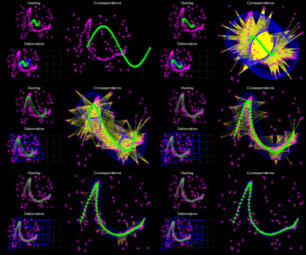
The thin plate spline robust point matching (TPS-RPM) algorithm by Chui and Rangarajan augments the RPM method to perform non-rigid registration by parametrizing the transformation as a thin plate spline.^[1] However, because the thin plate spline parametrization only exists in three dimensions, the method cannot be extended to problems involving four or more dimensions.

Kernel correlation

The kernel correlation (KC) approach of point set registration was introduced by Tsin and Kanade.^[6] Compared with ICP, the KC algorithm is more robust against noisy data. Unlike ICP, where, for every model point, only the closest scene point is considered, here every scene point affects every model point.^[6] As such this is a multiply-linked registration algorithm. For some kernel function $K$ , the kernel correlation $KC$ of two points $x_{i},x_{j}$ is defined thus:^[6]

$KC(x_{i},x_{j})=\int K(x,x_{i})\cdot K(x,x_{j})dx$

(kc.1)

The kernel function $K$ chosen for point set registration is typically symmetric and non-negative kernel, similar to the ones used in the Parzen window density estimation. The Gaussian kernel typically used for its simplicity, although other ones like the Epanechnikov kernel and the tricube kernel may be substituted.^[6] The kernel correlation of an entire point set ${\mathcal {\chi }}$ is defined as the sum of the kernel correlations of every point in the set to every other point in the set:^[6]

$KC({\mathcal {X}})=\sum _{i\neq j}KC(x_{i},x_{j})=2\sum _{i<j}KC(x_{i},x_{j})$

(kc.2)

The KC of a point set is proportional, within a constant factor, to the logarithm of the information entropy. Observe that the KC is a measure of a "compactness" of the point set—trivially, if all points in the point set were at the same location, the KC would evaluate to zero. The cost function of the point set registration algorithm for some transformation parameter $\theta$ is defined thus:

$\operatorname {cost} ({\mathcal {S}},{\mathcal {M}},\theta )=-\sum _{m\in {\mathcal {M}}}\sum _{s\in {\mathcal {S}}}KC(s,T(m,\theta ))$

(kc.3)

Some algebraic manipulation yields:

$KC({\mathcal {S}}\cup T({\mathcal {M}},\theta ))=KC({\mathcal {S}})+KC(T({\mathcal {M}},\theta ))-2\operatorname {cost} ({\mathcal {S}},{\mathcal {M}},\theta )$

(kc.4)

The expression is simplified by observing that $KC({\mathcal {S}})$ is independent of $\theta$ . Furthermore, assuming rigid registration, $KC(T({\mathcal {M}},\theta ))$ is invariant when $\theta$ is changed because the Euclidean distance between every pair of points stays the same under rigid transformation. So the above equation may be rewritten as:

$KC({\mathcal {S}}\cup T({\mathcal {M}},\theta ))=C-2\operatorname {cost} ({\mathcal {S}},{\mathcal {M}},\theta )$

(kc.5)

The kernel density estimates are defined as:

P_{\mathcal {M}}(x,\theta )={\frac {1}{N}}\sum _{m\in {\mathcal {M}}}K(x,T(m,\theta ))

P_{\mathcal {S}}(x)={\frac {1}{N}}\sum _{s\in {\mathcal {S}}}K(x,s)

The cost function can then be shown to be the correlation of the two kernel density estimates:

$\operatorname {cost} ({\mathcal {S}},{\mathcal {M}},\theta )=-N^{2}\int _{x}P_{\mathcal {M}}\cdot P_{\mathcal {S}}~dx$

(kc.6)

Having established the cost function, the algorithm simply uses gradient descent to find the optimal transformation. It is computationally expensive to compute the cost function from scratch on every iteration, so a discrete version of the cost function Equation (kc.6) is used. The kernel density estimates $P_{\mathcal {M}},P_{\mathcal {S}}$ can be evaluated at grid points and stored in a lookup table. Unlike the ICP and related methods, it is not necessary to find the nearest neighbour, which allows the KC algorithm to be comparatively simple in implementation.

Compared to ICP and EM-ICP for noisy 2D and 3D point sets, the KC algorithm is less sensitive to noise and results in correct registration more often.^[6]

Gaussian mixture model

The kernel density estimates are sums of Gaussians and may therefore be represented as Gaussian mixture models (GMM).^[11] Jian and Vemuri use the GMM version of the KC registration algorithm to perform non-rigid registration parametrized by thin plate splines.

Coherent point drift

Rigid (with the addition of scaling) registration of a blue point set

{\mathcal {M}}

to the red point set

{\mathcal {S}}

using the Coherent Point Drift algorithm. Both point sets have been corrupted with removed points and random spurious outlier points.

Affine registration of a blue point set

{\mathcal {M}}

to the red point set

{\mathcal {S}}

using the Coherent Point Drift algorithm.

Non-rigid registration of a blue point set

{\mathcal {M}}

to the red point set

{\mathcal {S}}

using the Coherent Point Drift algorithm. Both point sets have been corrupted with removed points and random spurious outlier points.

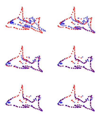
Coherent point drift (CPD) was introduced by Myronenko and Song.^[7]^[12] The algorithm takes a probabilistic approach to aligning point sets, similar to the GMM KC method. Unlike earlier approaches to non-rigid registration which assume a thin plate spline transformation model, CPD is agnostic with regard to the transformation model used. The point set ${\mathcal {M}}$ represents the Gaussian mixture model (GMM) centroids. When the two point sets are optimally aligned, the correspondence is the maximum of the GMM posterior probability for a given data point. To preserve the topological structure of the point sets, the GMM centroids are forced to move coherently as a group. The expectation maximization algorithm is used to optimize the cost function.^[7]

Let there be $M$ points in ${\mathcal {M}}$ and $N$ points in ${\mathcal {S}}$ . The GMM probability density function for a point $s$ is:

$p(s)=\sum _{i=1}^{M+1}P(i)p(s|i)$

(cpd.1)

where, in $D$ dimensions, $p(s|i)$ is the Gaussian distribution centered on point $m_{i}\in {\mathcal {M}}$ .

p(s|i)={\frac {1}{(2\pi \sigma ^{2})^{D/2)}}}\exp {\left(-{\frac {\lVert s-m_{i}\rVert ^{2}}{2\sigma ^{2}}}\right)}

The membership probabilities $P(i)={\frac {1}{M}}$ is equal for all GMM components. The weight of the uniform distribution is denoted as $w\in [0,1]$ . The mixture model is then:

$p(s)=w{\frac {1}{N}}+(1-w)\sum _{i=1}^{M}{\frac {1}{M}}p(s|i)$

(cpd.2)

The GMM centroids are re-parametrized by a set of parameters $\theta$ estimated by maximizing the likelihood. This is equivalent to minimizing the negative log-likelihood function:

$E(\theta ,\sigma ^{2})=-\sum _{j=1}^{N}\log \sum _{i=1}^{M+1}P(i)p(s|i)$

(cpd.3)

where it is assumed that the data is independent and identically distributed. The correspondence probability between two points $m_{i}$ and $s_{j}$ is defined as the posterior probability of the GMM centroid given the data point:

P(i|s_{j})={\frac {P(i)p(s_{j}|i)}{p(s_{j})}}

The expectation maximization (EM) algorithm is used to find $\theta$ and $\sigma ^{2}$ . The EM algorithm consists of two steps. First, in the E-step or estimation step, it guesses the values of parameters ("old" parameter values) and then uses Bayes' theorem to compute the posterior probability distributions $P^{\text{old}}(i,s_{j})$ of mixture components. Second, in the M-step or maximization step, the "new" parameter values are then found by minimizing the expectation of the complete negative log-likelihood function, i.e. the cost function:

$\operatorname {cost} =-\sum _{j=1}^{N}\sum _{i=1}^{M+1}P^{\text{old}}(i|s_{j})\log(P^{\text{new}}(i)p^{\text{new}}(s_{j}|i))$

(cpd.4)

Ignoring constants independent of $\theta$ and $\sigma$ , Equation (cpd.4) can be expressed thus:

$\operatorname {cost} (\theta ,\sigma ^{2})={\frac {1}{2\sigma ^{2}}}\sum _{j=1}^{N}\sum _{i=1}^{M+1}P^{\text{old}}(i|s_{j})\lVert s_{j}-T(m_{i},\theta )\rVert ^{2}+{\frac {N_{\mathbf {P} }D}{2}}\log {\sigma ^{2}}$

(cpd.5)

where

N_{\mathbf {P} }=\sum _{j=0}^{N}\sum _{i=0}^{M}P^{\text{old}}(i|s_{j})\leq N

with $N=N_{\mathbf {P} }$ only if $w=0$ . The posterior probabilities of GMM components computed using previous parameter values $P^{{{\text{old}}}}$ is:

$P^{\text{old}}(i|s_{j})={\frac {\exp \left(-{\frac {1}{2\sigma ^{{\text{old}}2}}}\lVert s_{j}-T(m_{i},\theta ^{\text{old}})\rVert ^{2}\right)}{\sum _{k=1}^{M}\exp \left(-{\frac {1}{2\sigma ^{{\text{old}}2}}}\lVert s_{j}-T(m_{k},\theta ^{\text{old}})\rVert ^{2}\right)+(2\pi \sigma ^{2})^{\frac {D}{2}}{\frac {w}{1-w}}{\frac {M}{N}}}}$

(cpd.6)

Minimizing the cost function in Equation (cpd.5) necessarily decreases the negative log-likelihood function $E$ in Equation (cpd.3) unless it is already at a local minimum.^[7] Thus, the algorithm can be expressed using the following pseudocode, where the point sets ${\mathcal {M}}$ and ${\mathcal {S}}$ are represented as $M\times D$ and $N\times D$ matrices $\mathbf {M}$ and $\mathbf {S}$ respectively:^[7]

   Algorithm CPD $({\mathcal {M}},{\mathcal {S}})$ 
        $\theta :=\theta _{0}$ 
       initialize  $0\leq w\leq 1$ 
        $\sigma ^{2}:={\frac {1}{DNM}}\sum _{j=1}^{N}\sum _{i=1}^{M}\lVert s_{j}-m_{i}\rVert ^{2}$ 
       while not registered:
           // E-step, compute  $P$ 
           for  $i\in [1,M]$  and  $j\in [1,N]$ :
                $p_{ij}:={\frac {\exp \left(-{\frac {1}{2\sigma ^{2}}}\lVert s_{j}-T(m_{i},\theta )\rVert ^{2}\right)}{\sum _{k=1}^{M}\exp \left(-{\frac {1}{2\sigma ^{2}}}\lVert s_{j}-T(m_{k},\theta )\rVert ^{2}\right)+(2\pi \sigma ^{2})^{\frac {D}{2}}{\frac {w}{1-w}}{\frac {M}{N}}}}$ 
           // M-step, solve for optimal transformation
            $\lbrace \theta ,\sigma ^{2}\rbrace :=\mathbf {solve} (\mathbf {S} ,\mathbf {M} ,\mathbf {P} )$ 
       return  $θ$

where the vector $\mathbf {1}$ is a column vector of ones. The solve function differs by the type of registration performed. For example, in rigid registration, the output is a scale $a$ , a rotation matrix $\mathbf {R}$ , and a translation vector $\mathbf {t}$ . The parameter $\theta$ can be written as a tuple of these:

\theta =\lbrace a,\mathbf {R} ,\mathbf {t} \rbrace

which is initialized to one, the identity matrix, and a column vector of zeroes:

\theta _{0}=\lbrace 1,\mathbf {I} ,\mathbf {0} \rbrace

The aligned point set is:

T(\mathbf {M} )=a\mathbf {M} \mathbf {R} ^{T}+\mathbf {1} \mathbf {t} ^{T}

The solve_rigid function for rigid registration can then be written as follows, with derivation of the algebra explained in Myronenko's 2010 paper.^[7]

   solve_rigid $(\mathbf {S} ,\mathbf {M} ,\mathbf {P} )$ 
        $N_{\mathbf {P} }:=\mathbf {1} ^{T}\mathbf {P} \mathbf {1}$ 
        $\mu _{s}:={\frac {1}{N_{\mathbf {P} }}}\mathbf {S} ^{T}\mathbf {P} ^{T}\mathbf {1}$ 
        $\mu _{m}:={\frac {1}{N_{\mathbf {P} }}}\mathbf {M} ^{T}\mathbf {P} \mathbf {1}$ 
        ${\hat {\mathbf {S} }}:=\mathbf {S} -\mathbf {1} \mu _{s}^{T}$ 
        ${\hat {\mathbf {M} }}:=\mathbf {M} -\mathbf {1} \mu _{m}^{T}$ 
        $\mathbf {A} :={\hat {\mathbf {S} ^{T}}}\mathbf {P} ^{T}{\hat {\mathbf {M} }}$ 
        $\mathbf {U} ,\mathbf {V} :=\mathbf {svd} (\mathbf {A} )$  // the singular value decomposition of  $\mathbf {A} =\mathbf {U} \Sigma \mathbf {V} ^{T}$ 
        $\mathbf {C} :=\operatorname {diag} (1,...,1,\det(\mathbf {UV} ^{T}))$  //  $diag(ξ)$  is the diagonal matrix formed from vector  $ξ$ 
        $\mathbf {R} :=\mathbf {UCV} ^{T}$ 
        $a:={\frac {\operatorname {tr} (\mathbf {A} ^{T}\mathbf {R} )}{\operatorname {tr} (\mathbf {{\hat {\mathbf {M} }}^{T}\operatorname {diag} (\mathbf {P} \mathbf {1} ){\hat {\mathbf {M} }}} )}}$  //  $tr$  is the trace of a matrix
        $\mathbf {t} :=\mu _{s}-a\mathbf {R} \mu _{m}$ 
        $\sigma ^{2}:={\frac {1}{N_{\mathbf {P} }D}}(\operatorname {tr} (\mathbf {{\hat {\mathbf {S} }}^{T}\operatorname {diag} (\mathbf {P} ^{T}\mathbf {1} ){\hat {\mathbf {S} }}} ))-a\operatorname {tr} (\mathbf {A} ^{T}\mathbf {R} )$ 
       return  $\lbrace a,\mathbf {R} ,\mathbf {t} \rbrace ,\sigma ^{2}$

For affine registration, where the goal is to find an affine transformation instead of a rigid one, the output is an affine transformation matrix $\mathbf {B}$ and a translation $\mathbf {t}$ such that the aligned point set is:

T(\mathbf {M} )=\mathbf {M} \mathbf {B} ^{T}+\mathbf {1} \mathbf {t} ^{T}

The solve_affine function for rigid registration can then be written as follows, with derivation of the algebra explained in Myronenko's 2010 paper.^[7]

   solve_affine $(\mathbf {S} ,\mathbf {M} ,\mathbf {P} )$ 
        $N_{\mathbf {P} }:=\mathbf {1} ^{T}\mathbf {P} \mathbf {1}$ 
        $\mu _{s}:={\frac {1}{N_{\mathbf {P} }}}\mathbf {S} ^{T}\mathbf {P} ^{T}\mathbf {1}$ 
        $\mu _{m}:={\frac {1}{N_{\mathbf {P} }}}\mathbf {M} ^{T}\mathbf {P} \mathbf {1}$ 
        ${\hat {\mathbf {S} }}:=\mathbf {S} -\mathbf {1} \mu _{s}^{T}$ 
        ${\hat {\mathbf {M} }}:=\mathbf {M} -\mathbf {1} \mu _{s}^{T}$ 
        $\mathbf {B} :=({\hat {\mathbf {S} ^{T}}}\mathbf {P} ^{T}{\hat {\mathbf {M} }})({\hat {\mathbf {M} ^{T}}}\operatorname {diag} (\mathbf {P} \mathbf {1} ){\hat {\mathbf {M} }})^{-1}$ 
        $\mathbf {t} :=\mu _{s}-\mathbf {B} \mu _{m}$ 
        $\sigma ^{2}:={\frac {1}{N_{\mathbf {P} }D}}(\operatorname {tr} (\mathbf {{\hat {\mathbf {S} }}\operatorname {diag} (\mathbf {P} ^{T}\mathbf {1} ){\hat {\mathbf {S} }}} )-\operatorname {tr} ({\hat {\mathbf {S} ^{T}}}\mathbf {P} ^{T}{\hat {\mathbf {M} }}\mathbf {B} ^{T}))$ 
       return  $\{\mathbf {B} ,\mathbf {t} \},\sigma ^{2}$

It is also possible to use CPD with non-rigid registration using a parametrization derived using calculus of variation.^[7]

Sums of Gaussian distributions can be computed in linear time using the fast Gauss transform (FGT).^[7] Consequently, the time complexity of CPD is $O(M+N)$ , which is asymptotically much faster than $O(MN)$ methods.^[7]

External links

References

1 2 3 4 Chui, Haili; Rangarajan, Anand (2003). "A new point matching algorithm for non-rigid registration". Computer Vision and Image Understanding. 89 (2): 114–141. doi:10.1016/S1077-3142(03)00009-2.
1 2 3 Fitzgibbon, Andrew W. (2003). "Robust registration of 2D and 3D point sets". Image and Vision Computing. 21 (13): 1145–1153. doi:10.1016/j.imavis.2003.09.004.
↑ Hill, Derek LG; Hawkes, D. J.; Crossman, J. E.; Gleeson, M. J.; Cox, T. C. S.; Bracey, E. E. C. M. L.; Strong, A. J.; Graves, P. (1991). "Registration of MR and CT images for skull base surgery using point-like anatomical features". British journal of radiology. 64 (767): 1030–1035. doi:10.1259/0007-1285-64-767-1030.
↑ Studholme, C.; Hill, D. L.; Hawkes, D. J. (1995). Automated 3D Registration of Truncated MR and CT Images of the Head. Proceedings of the Sixth British Machine Vision Conference. pp. 27–36.
1 2 Jian, Bing; Vemuri, Baba C. (2011). "Robust Point Set Registration Using Gaussian Mixture Models". IEEE Transactions on Pattern Analysis and Machine Intelligence. 33 (8): 1633–1645. doi:10.1109/tpami.2010.223.
1 2 3 4 5 6 7 8 9 10 Tsin, Yanghai; Kanade, Takeo (2004). "A Correlation-Based Approach to Robust Point Set Registration". Computer Vision ECCV. Springer Berlin Heidelberg: 558–569. doi:10.1007/978-3-540-24672-5_44.
1 2 3 4 5 6 7 8 9 10 11 12 Myronenko, Andriy; Song, Xubo (2010). "Point set registration: Coherent Point drift". IEEE Transactions on Pattern Analysis and Machine Intelligence. 32 (2): 2262–2275. doi:10.1109/tpami.2010.46.
↑ Besl, Paul; McKay, Neil (1992). "A Method for Registration of 3-D Shapes". IEEE Transactions on Pattern Analysis and Machine Intelligence. 14 (2): 239–256. doi:10.1109/34.121791.
↑ Rusinkiewicz, Szymon; Levoy, Marc (2001). Efficient variants of the ICP algorithm. Proceedings of the Third International Conference on 3-D Digital Imaging and Modeling, 2001. IEEE. pp. 145–152. doi:10.1109/IM.2001.924423.
1 2 3 4 5 Gold, Steven; Rangarajan, Anand; Lu, Chien-Ping; Suguna, Pappu; Mjolsness, Eric (1998). "New algorithms for 2d and 3d point matching:: pose estimation and correspondence". Pattern Recognition. 38 (8): 1019–1031. doi:10.1016/S0031-3203(98)80010-1.
↑ Jian, Bing; Vemuri, Baba C. (2005). A robust algorithm for point set registration using mixture of Gaussians. Tenth IEEE International Conference on Computer Vision 2005. 2. pp. 1246–1251.
↑ Myronenko, Andriy; Song, Xubo; Carriera-Perpinán, Miguel A. (2006). "Non-rigid point set registration: Coherent point drift". Advances in Neural Information Processing Systems. 19: 1009–1016. Retrieved 31 May 2014.

This article is issued from Wikipedia - version of the 8/1/2016. The text is available under the Creative Commons Attribution/Share Alike but additional terms may apply for the media files.