Łukaszyk–Karmowski metric

In mathematics, the Łukaszyk–Karmowski metric is a function defining a distance between two random variables or two random vectors.^[1]^[2] This function is not a metric as it does not satisfy the identity of indiscernibles condition of the metric, that is for two identical arguments its value is greater than zero. The concept is named after Szymon Łukaszyk and Wojciech Karmowski.

Continuous random variables

The Łukaszyk–Karmowski metric D between two continuous independent random variables X and Y is defined as:

D(X, Y) = \int_{-\infty}^\infty \int_{-\infty}^\infty |x-y|f(x)g(y) \, dx\, dy

where f(x) and g(y) are the probability density functions of X and Y respectively.

One may easily show that such metrics above do not satisfy the identity of indiscernibles condition required to be satisfied by the metric of the metric space. In fact they satisfy this condition if and only if both arguments X, Y are certain events described by Dirac delta density probability distribution functions. In such a case:

D_{\delta\delta}(X, Y) = \int_{-\infty}^\infty \int_{-\infty}^\infty |x-y|\delta(x-\mu_x)\delta(y-\mu_y) \, dx\, dy = |\mu_x-\mu_y|

the Łukaszyk–Karmowski metric simply transforms into the metric between expected values $\mu _{x}$ , $\mu _{y}$ of the variables X and Y and obviously:

D_{\delta\delta}(X, X) = |\mu_x-\mu_x| = 0.

For all the other cases however:

D\left(X, X\right) > 0. \,

The Łukaszyk–Karmowski metric satisfies the remaining non-negativity and symmetry conditions of metric directly from its definition (symmetry of modulus), as well as subadditivity/triangle inequality condition:

\begin{align} &{} D(X, Z) = \int_{-\infty}^\infty \int_{-\infty}^\infty |x-z|f(x)h(z) \, dx\, dz\ = \int_{-\infty}^\infty \int_{-\infty}^\infty |x-z|f(x)h(z) \, dx\, dz \int_{-\infty}^\infty g(y) dy\ \\ &{} = \int_{-\infty}^\infty \int_{-\infty}^\infty \int_{-\infty}^\infty |(x-y)+(y-z)|f(x)g(y)h(z) \, dx\, dy\, dz\ \\ &{} \le \int_{-\infty}^\infty \int_{-\infty}^\infty \int_{-\infty}^\infty (|x-y|+|y-z|)f(x)g(y)h(z) \, dx\, dy\, dz\ \\ &{} = \int_{-\infty}^\infty \int_{-\infty}^\infty \int_{-\infty}^\infty |x-y|f(x)g(y)h(z) \, dx\, dy\, dz\ + \int_{-\infty}^\infty \int_{-\infty}^\infty \int_{-\infty}^\infty |y-z|f(x)g(y)h(z) \, dx\, dy\, dz\ \\ &{} = \int_{-\infty}^\infty \int_{-\infty}^\infty |x-y|f(x)g(y) \, dx\, dy\ + \int_{-\infty}^\infty \int_{-\infty}^\infty |y-z|g(y)h(z) \, dy\, dz\ \\ &{} = D(X, Y) + D(Y, Z) \end{align}

Thus

D(X, Z) \le D(X, Y)+D(Y, Z). \,

L–K metric between two random variables X and Y having normal distributions and the same standard deviation

\sigma = 0, \sigma = 0.2, \sigma = 0.4, \sigma = 0.6, \sigma = 0.8, \sigma = 1

(starting with the bottom curve).

m_{xy} = |\mu_x-\mu_y|

denotes a distance between means of X and Y.

In the case where X and Y are dependent on each other, having a joint probability density function f(x, y), the L–K metric has the following form:

\int_{-\infty}^\infty \int_{-\infty}^\infty |x-y| f(x, y) \, dx\, dy.

Example: two continuous random variables with normal distributions (NN)

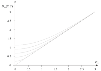
If both random variables X and Y have normal distributions with the same standard deviation σ, and if moreover X and Y are independent, then D(X, Y) is given by

D_{NN}(X, Y) = \mu_{xy} + \frac{2\sigma}{\sqrt\pi}\operatorname{exp}\left(-\frac{\mu_{xy}^2}{4\sigma^2}\right)-\mu_{xy} \operatorname{erfc} \left(\frac{\mu_{xy}}{2\sigma}\right) ,

where

\mu_{xy} = \left|\mu_x-\mu_y\right|,

where erfc(x) is the complementary error function and where the subscripts NN indicate the type of the L–K metric.

In this case, the lowest possible value of the function $D_{NN}(X, Y)$ is given by

\lim_{\mu_{xy}\to 0} D_{NN}(X, Y) = D_{NN}(X, X) = \frac{2\sigma}{\sqrt\pi}.

Example: two continuous random variables with uniform distributions (RR)

When both random variables X and Y have uniform distributions (R) of the same standard deviation σ, D(X, Y) is given by

D_{RR}(X, Y) = \begin{cases} \frac{24\sqrt{3}\sigma^3-\mu_{xy}^3+6\sqrt{3}\sigma\mu_{xy}^2}{36\sigma^2}, & \mu_{xy}<2\sqrt{3}\sigma, \\ \mu_{xy}, & \mu_{xy} \ge 2\sqrt{3}\sigma. \end{cases}

The minimal value of this kind of L–K metric is

D_{RR}(X, X) = \frac{2\sigma}{\sqrt{3}}.

Discrete random variables

In case the random variables X and Y are characterized by discrete probability distribution the Łukaszyk–Karmowski metric D is defined as:

D(X, Y) = \sum_{i} \sum_{j} |x_i-y_j|P(X=x_i)P(Y=y_j).\,

For example for two discrete Poisson-distributed random variables X and Y the equation above transforms into:

D_{PP}(X, Y) = \sum_{x=0}^n\sum_{y=0}^n |x-y|\frac{{\lambda_x}^x{\lambda_y}^ye^{-(\lambda_x+\lambda_y)}}{x!y!}.

Random vectors

equidistant surface for Euclidean metric

d^{2}(\mathbf{x},\mathbf{0})=\sqrt{x_{1}^2+x_{2}^2}

equidistant surface for Euclidean L–K metric

D_{R\delta}^{2}(\mathbf{X},\mathbf{0}) \left( \left(\mathbf{X,0}\right): \Omega \to \mathbb{R}^2 \right)

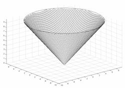
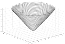
The Łukaszyk–Karmowski metric of random variables may be easily extended into metric D(X, Y) of random vectors X, Y by substituting $|x-y|$ with any metric operator d(x,y):

D(\mathbf{X}, \mathbf{Y}) =\int_{\Omega} \int_{\Omega} d(\mathbf{x}, \mathbf{y})F(\mathbf{x})G(\mathbf{y})\, d\Omega_x \, d\Omega_y.

For example substituting d(x,y) with an Euclidean metric and assuming two-dimensionality of random vectors X, Y would yield:

D(\mathbf{X}, \mathbf{Y}) =\int_{\Omega} \int_\Omega \sqrt{\sum_{i=1}^2|x_i-y_i|^2} F( x_1, x_2)G(y_1, y_2) \, dx_1\, dx_2\, dy_1\, dy_2.

This form of L–K metric is also greater than zero for the same vectors being measured (with the exception of two vectors having Dirac delta coefficients) and satisfies non-negativity and symmetry conditions of metric. The proofs are analogous to the ones provided for the L–K metric of random variables discussed above.

In case random vectors X and Y are dependent on each other, sharing common joint probability distribution F(X, Y) the L–K metric has the form:

D(\mathbf{X}, \mathbf{Y}) =\int_{\Omega} \int_{\Omega} d(\mathbf{x}, \mathbf{y})F(\mathbf{x}, \mathbf{y}) \, d\Omega_x \, d \Omega_y.

Random vectors – the Euclidean form

If the random vectors X and Y are not also only mutually independent but also all components of each vector are mutually independent, the Łukaszyk–Karmowski metric for random vectors is defined as:

D_{**}^{(p)}(\mathbf{X}, \mathbf{Y}) = \left( {\sum_i{D_{**}(X_i, Y_i)}^p} \right)^{\frac1p}

where:

D_{**}(X_i, Y_i)\,

is a particular form of L–K metric of random variables chosen in dependence of the distributions of particular coefficients $X_{i}$ and $Y_{i}$ of vectors X, Y .

Such a form of L–K metric also shares the common properties of all L–K metrics.

It does not satisfy the identity of indiscernibles condition:

\forall{\mathbf{X}, \mathbf{Y}}\ D_{**}^{(p)}(\mathbf{X}, \mathbf{Y}) = 0 \ \nLeftrightarrow \ \mathbf{X} = \mathbf{Y} \,

since:

D_{**}^{(p)}(\mathbf{X}, \mathbf{X}) = 0 \Leftrightarrow \ \forall{i} \ D_{**}(X_i, X_i) = 0

but from the properties of L–K metric for random variables it follows that:

\exists\ X_i\ D_{**}(X_i, X_i) > 0

It is non-negative and symmetric since the particular coefficients are also non-negative and symmetric:

\forall\ i \ D_{**}(X_i, Y_i) > 0 \,

\forall\ i \ D_{**}(X_i, Y_i) = D_{**}(Y_i, X_i)

It satisfies the triangle inequality:

\forall\ \mathbf{X}, \mathbf{Y}, \mathbf{Z} \ D_{**}^{(p)}(\mathbf{X}, \mathbf{Z}) \le D_{**}^{(p)}(\mathbf{X}, \mathbf{Y}) + D_{**}^{(p)}(\mathbf{Y}, \mathbf{Z})

since (cf. Minkowski inequality):

\begin{align} &{} \left( {\sum_i{D_{**}(X_i, Y_i)}^p} \right)^{\frac1p} + \left( {\sum_i{D_{**}(Y_i, Z_i)}^p} \right)^{\frac1p}\ \ge \\ &{} \ge \left( {\sum_i{D_{**}(X_i, Y_i) + D_{**}(Y_i, Z_i)}^p} \right)^{\frac1p} \ge \\ &{} \ge \left( {\sum_i{D_{**}(X_i, Z_i)}^p} \right)^{\frac1p} \end{align}

Physical interpretation

The Łukaszyk–Karmowski metric may be considered as a distance between quantum mechanics particles described by wavefunctions ψ, where the probability dP that given particle is present in given volume of space dV amounts:

dP = |\psi(x, y, z)|^2 dV. \,

A quantum particle in a box

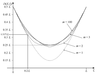
L–K metric between a quantum particle in a one-dimensional box of length L and a given point ξ of the box

(0 \le \xi \le L)

For example the wavefunction of a quantum particle (X) in a box of length L has the form:

\psi_m(x) = \sqrt{\frac{2}{L}} \sin{\left(\frac{m \pi x}{L} \right)}, \,

In this case the L–K metric between this particle and any point $\xi \in (0, L)\,$ of the box amounts:

\begin{align} &{} D(X, \xi) = \int\limits_{0}^L |x-\xi||\psi_m(x)|^2dx = \\ &{} = \frac{\xi^2}{L} - \xi +L\left(\frac{1}{2}-\frac{\sin^2(\frac{m\pi\xi}{L})}{m^2\pi^2}\right). \end{align}

From the properties of the L–K metric it follows that the sum of distances between the edge of the box (ξ = 0 or ξ= L) and any given point and the L–K metric between this point and the particle X is greater than L–K metric between the edge of the box and the particle. E.g. for a quantum particle X at an energy level m = 2 and point ξ = 0.2:

d(0,0.2L) + D(0.2L, X) \approx 0.2L + 0.3171L = 0.517L \neq D(0, X) = 0.5L = d(0,0.5L).\,

Obviously the L–K metric between the particle and the edge of the box (D(0, X) or D(L, X)) amounts 0.5L and is independent on the particle's energy level.

Two quantum particles in a box

A distance between two particles bouncing in a one-dimensional box of length L having time-independent wavefunctions:

\psi_m(x) = \sqrt{\frac{2}{L}} \sin{\left(\frac{m \pi x}{L} \right)}, \,

\psi_n(y) = \sqrt{\frac{2}{L}} \sin{\left(\frac{n \pi y}{L} \right)}, \,

may be defined in terms of Łukaszyk–Karmowski metric of independent random variables as:

\begin{align} &{} D(X, Y) = \int\limits_{0}^L \int\limits_0^L |x-y||\psi_m(x)|^2|\psi_n(y)|^2 \, dx\, dy \\ &{} = \begin{cases} L\left(\frac{4 \pi^2 m^2 -15}{12\pi^2m^2} \right) & m=n, \\ L\left(\frac{2 \pi^2 m^2 n^2 -3m^2 - 3n^2}{6\pi^2m^2n^2} \right) & m \neq n \end{cases}\end{align}

The distance between particles X and Y is minimal for m = 1 i n = 1, that is for the minimum energy levels of these particles and amounts:

\min(D(X, Y)) = L\left(\frac{4 \pi^2-15}{12\pi^2} \right) \approx 0.2067L. \,

According to properties of this function, the minimum distance is nonzero. For greater energy levels m, n it approaches to L/3.

Popular explanation

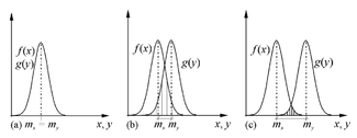
Normal distributions of two random variables X and Y of the same variance for three locations of their means µ_x, µ_y

Suppose we have to measure the distance between point µ_x and point µ_y, which are collinear with some point 0. Suppose further that we instructed this task to two independent and large groups of surveyors equipped with tape measures, wherein each surveyor of the first group will measure distance between 0 and µ_x and each surveyor of the second group will measure distance between 0 and µ_y.

Under the following assumptions we may consider the two sets of received observations x_i, y_j as random variables X and Y having normal distribution of the same variance σ² and distributed over "factual locations" of points µ_x, µ_y.

Calculating the arithmetic mean for all pairs |x_i − y_j| we should then obtain the value of L–K metric D_NN(X, Y). Its characteristic curvilinearity arises from the symmetry of modulus and overlapping of distributions f(x), g(y) when their means approach each other.

An interesting experiment the results of which coincide with the properties of L–K metric was performed in 1967 by Robert Moyer and Thomas Landauer who measured the precise time an adult took to decide which of two Arabic digits was the largest. When the two digits were numerically distanced such as 2 and 9. subjects responded quickly and accurately. But their response time slowed by more than 100 milliseconds when they were closer such as 5 and 6, and subjects then erred as often as once in every ten trials. The distance effect was present both among highly intelligent persons, as well as those who were trained to escape it.^[3]

Practical applications

A Łukaszyk–Karmowski metric may be used instead of a metric operator (commonly the Euclidean distance) in various numerical methods, and in particular in approximation algorithms such us radial basis function networks ,^[4]^[5] inverse distance weighting or Kohonen self-organizing maps.

This approach is physically based, allowing the real uncertainty in the location of the sample points to be considered. ^[6]^[7]

References

↑ Metryka Pomiarowa, przykłady zastosowań aproksymacyjnych w mechanice doświadczalnej (Measurement metric, examples of approximation applications in experimental mechanics), PhD thesis, Szymon Łukaszyk (author), Wojciech Karmowski (supervisor), Tadeusz Kościuszko Cracow University of Technology, submitted December 31, 2001, completed March 31, 2004
↑ A new concept of probability metric and its applications in approximation of scattered data sets, Łukaszyk Szymon, Computational Mechanics Volume 33, Number 4, 299–304, Springer-Verlag 2003 doi:10.1007/s00466-003-0532-2
↑ The Number Sense: How the Mind Creates Mathematics, Stanislas Dehaene, Oxford University Press US, 1999, ISBN 0-19-513240-8, pp. 73–75
↑ Taher Zaki, Driss Mammass, Abdellatif Ennaji, Fathallah Nouboud (2010) Classification of Arabic Documents by a Model of Fuzzy Proximity with a Radial Basis Function, International Journal of Future Generation Communication and Networking, 3 (4), p. 34
↑ Florian Hogewind, Peter Bissolli (2010) Operational maps of monthly mean temperature for WMO-Region VI (Europe and Middle East), IDŐJÁRÁS, Quarterly Journal of the Hungarian Meteorological Service, Vol. 115, No. 1-2, January–June 2011, pp. 31-49, p. 41
↑ Gang Meng, Jane Law, Mary E. Thompson (2010) "Small-scale health-related indicator acquisition using secondary data spatial interpolation", International Journal of Health Geographics, 9:50 doi:10.1186/1476-072X-9-50
↑ Gang Meng (2010)Social and Spatial Determinants of Adverse Birth Outcome Inequalities in Socially Advanced Societies, Thesis (Doctor of Philosophy in Planning), University of Waterloo, Canada,

This article is issued from Wikipedia - version of the 10/20/2016. The text is available under the Creative Commons Attribution/Share Alike but additional terms may apply for the media files.